Using Functional Dependency Analysis to improve Join performance

Two months ago I talked about how we got 4 9s of correctness in sqllogictests. I mentioned how the most time consuming task was optimizing a test query that joined 64 tables, a query that even MySQL choked on. I'm going to dive deeper into how we actually solved this problem, and how the our fix can improve the performance of real user-written queries.
As a refresher, this is the query that neither Dolt nor MySQL was able to efficiently evaluate:
  SELECT x46,x59,x60,x24,x5,x28,x17,x19,x36,x51,x30,x25,x48,x31,x63,x7,x20,x10,x27,x32,x62,x21,x14,x15,x58,x50,x13,x43,x56,x12,x40,x41,x6,x45,x23,x54,x37,x8,x3,x22,x34,x29,x33,x55,x38,x26,x39,x35,x18,x52,x1,x2,x4,x11,x47,x44,x61,x49,x53,x64,x57,x42,x9,x16
    FROM t17,t7,t30,t12,t49,t23,t63,t51,t33,t43,t9,t62,t21,t48,t36,t1,t4,t25,t6,t35,t52,t58,t50,t14,t32,t53,t22,t13,t15,t10,t19,t61,t5,t11,t40,t29,t46,t31,t60,t55,t54,t16,t42,t2,t20,t39,t8,t38,t44,t41,t56,t64,t37,t59,t34,t3,t24,t57,t18,t45,t26,t27,t47,t28
   WHERE a49=b21 AND b32=a16 AND a62=b15 AND b43=a26 AND b27=a54 AND a57=b34 AND b44=a35 AND a51=b8 AND b56=a31 AND a33=b63 AND b37=a10 AND a21=b16 AND b23=a7 AND a37=b7 AND a32=b50 AND a6=b39 AND a14=b47 AND b9=a25 AND a27=b6 AND a29=b40 AND a60=b36 AND b64=a45 AND b46=a36 AND a39=b41 AND b61=a64 AND b17=a50 AND a63=b14 AND a18=b25 AND b29=a2 AND b58=a24 AND a28=b42 AND a12=b57 AND a56=b2 AND a4=b1 AND b19=a8 AND a41=b48 AND a61=b52 AND a40=b20 AND a3=b62 AND a11=b33 AND a23=b26 AND a34=b28 AND b60=a52 AND a31=10 AND b30=a59 AND b53=a47 AND b5=a55 AND b18=a43 AND b3=a44 AND a13=b24 AND a46=b35 AND a30=b51 AND a17=b59 AND b54=a5 AND a38=b4 AND a53=b55 AND b22=a20 AND a19=b38 AND b13=a42 AND a58=b49 AND a1=b45 AND b12=a48 AND a15=b10 AND a22=b11
It's a join of 64 tables. The data being queried was actually quite small: each of the individual tables only had ten rows and two columns, so the entire database totaled only a couple of kilobytes. Yet our measurements suggested that it would take both Dolt and MySQL millions of years to evaluate.
If you run the same query in Dolt today, it takes under a second:
  +------------------+-----------------+-----------------+-----------------+----------------+-----------------+------------------+-----------------+-----------------+-----------------+-----------------+-----------------+-----------------+------------------+-----------------+----------------+-----------------+-----------------+-----------------+------------------+-----------------+------------------+-----------------+-----------------+------------------+------------------+-----------------+-----------------+-----------------+-----------------+-----------------+-----------------+----------------+-----------------+-----------------+-----------------+-----------------+----------------+----------------+-----------------+-----------------+-----------------+-----------------+-----------------+-----------------+-----------------+------------------+-----------------+-----------------+-----------------+----------------+----------------+----------------+-----------------+-----------------+-----------------+-----------------+-----------------+-----------------+-----------------+-----------------+------------------+----------------+-----------------+
  | x46              | x59             | x60             | x24             | x5             | x28             | x17              | x19             | x36             | x51             | x30             | x25             | x48             | x31              | x63             | x7             | x20             | x10             | x27             | x32              | x62             | x21              | x14             | x15             | x58              | x50              | x13             | x43             | x56             | x12             | x40             | x41             | x6             | x45             | x23             | x54             | x37             | x8             | x3             | x22             | x34             | x29             | x33             | x55             | x38             | x26             | x39              | x35             | x18             | x52             | x1             | x2             | x4             | x11             | x47             | x44             | x61             | x49             | x53             | x64             | x57             | x42              | x9             | x16             |
  +------------------+-----------------+-----------------+-----------------+----------------+-----------------+------------------+-----------------+-----------------+-----------------+-----------------+-----------------+-----------------+------------------+-----------------+----------------+-----------------+-----------------+-----------------+------------------+-----------------+------------------+-----------------+-----------------+------------------+------------------+-----------------+-----------------+-----------------+-----------------+-----------------+-----------------+----------------+-----------------+-----------------+-----------------+-----------------+----------------+----------------+-----------------+-----------------+-----------------+-----------------+-----------------+-----------------+-----------------+------------------+-----------------+-----------------+-----------------+----------------+----------------+----------------+-----------------+-----------------+-----------------+-----------------+-----------------+-----------------+-----------------+-----------------+------------------+----------------+-----------------+
  | table t46 row 10 | table t59 row 2 | table t60 row 6 | table t24 row 9 | table t5 row 7 | table t28 row 4 | table t17 row 10 | table t19 row 8 | table t36 row 3 | table t51 row 7 | table t30 row 9 | table t25 row 1 | table t48 row 2 | table t31 row 10 | table t63 row 9 | table t7 row 2 | table t20 row 4 | table t10 row 8 | table t27 row 6 | table t32 row 10 | table t62 row 9 | table t21 row 10 | table t14 row 3 | table t15 row 9 | table t58 row 10 | table t50 row 10 | table t13 row 1 | table t43 row 9 | table t56 row 9 | table t12 row 2 | table t40 row 7 | table t41 row 9 | table t6 row 8 | table t45 row 6 | table t23 row 3 | table t54 row 2 | table t37 row 5 | table t8 row 5 | table t3 row 9 | table t22 row 4 | table t34 row 4 | table t29 row 6 | table t33 row 3 | table t55 row 1 | table t38 row 8 | table t26 row 9 | table t39 row 10 | table t35 row 8 | table t18 row 7 | table t52 row 9 | table t1 row 7 | table t2 row 3 | table t4 row 6 | table t11 row 5 | table t47 row 8 | table t44 row 1 | table t61 row 9 | table t49 row 2 | table t53 row 1 | table t64 row 3 | table t57 row 5 | table t42 row 10 | table t9 row 8 | table t16 row 8 |
  +------------------+-----------------+-----------------+-----------------+----------------+-----------------+------------------+-----------------+-----------------+-----------------+-----------------+-----------------+-----------------+------------------+-----------------+----------------+-----------------+-----------------+-----------------+------------------+-----------------+------------------+-----------------+-----------------+------------------+------------------+-----------------+-----------------+-----------------+-----------------+-----------------+-----------------+----------------+-----------------+-----------------+-----------------+-----------------+----------------+----------------+-----------------+-----------------+-----------------+-----------------+-----------------+-----------------+-----------------+------------------+-----------------+-----------------+-----------------+----------------+----------------+----------------+-----------------+-----------------+-----------------+-----------------+-----------------+-----------------+-----------------+-----------------+------------------+----------------+-----------------+
  1 row in set (0.11 sec)
How did we accomplish this? To answer that, we need to understand what makes join queries slow in the first place.
If you're already familiar with how SQL engines evaluate joins and common tricks to speed them up, feel free to skip ahead to [].
Why are Joins Slow?
Consider the following example database and query: we have a database containing every game ever played in a hypothetical sports conference. The database schema looks like this:
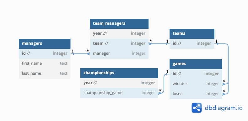
For those who prefer SQL, here's the CREATE TABLE statements used:
  > show create table managers;
  create table managers (id int primary key, first_name text, last_name text);

  > select count(*) from managers;
  1K

  > show create table team_managers;
  create table team_managers(year int, team int, manager int,
      primary key (year, team),
      unique key (team, manager),
      foreign key (manager) references managers(id),
      foreign key (team) references teams(id));

  > select count(*) from team_managers;
  10K

  > show create table championships;
  create table championships(year int primary key, championship_game int,
      foreign key (championship_game) references games(id));

  > select count(*) from championships;
  10

  > show create table games;
  create table games(id int primary key, winner int, loser int,
  foreign key (winner) references teams(id),
  foreign key (loser) references teams(id));

  > select count(*) from games;
  100M
It's a big conference: there's a thousand teams, and a thousand managers. But it's also a young conference: there have only been ten years of tournaments. Still, these teams play a lot of games: our table has one hundred million recorded games.
Suppose we want to get the name of every manager whose team has won a championship. We might write a query like this:
  select distinct first_name, last_name from managers
  	join team_managers on managers.id = team_managers.manager
      join games on team_managers.team = games.winner
      join championships on team_managers.year = championships.year
      	and games.id = championships.championship_game;
Without optimizations, this query falls afoul of two related but distinct pitfalls: large intermediate result sets, and poor physical planning. Either one of these is enough to slow a join to a crawl. Having both is catastrophic.
Intermediate Result Sets
When a statement contains multiple joins, typically the result of each join gets used as the input for the next join.
Then, if the query consists of multiple joins, then every pair of rows that passes the first join condition will get fed into the next one, and get paired with each row in yet another table. If we're lucky, then the first join will weed out most of the possible row combinations, and all the subsequent joins will be fast. But if we're unlucky, then the number of candidates at each step grows exponentially.
Let's look at how many rows will be generated by each join in the query.
First join:
managers join team_managers on managers.id = team_managers.manager
- Rows in left table: 1K
- Rows in right table: 10K
- Total pairs: 10M
- Pairs that match the condition: 10K
Second join:
... join games on team_managers.team = games.winner
- Rows in left table: 10K
- Rows in right table: 100M
- Total pairs: 1T
- Pairs that match the condition: 100M
Third join:
...join games on games.id = championships.championship_game and games.winner = team_managers.team;
- Rows in left table: 100M
- Rows in right table: 10
- Total pairs: 1B
- Pairs that match the condition: 10
So even though there are only ten rows in the final result, at one point we were looking at one trillion possible candidates. And the second join had one hundred million results.
Physical Join Planning
A physical join plan refers to the actual algorithm used to evaluate a single join expression. I previously wrote about the different physical joins within Dolt, including one that we designed ourselves. Join planning is the act of choosing the best physical plan for each join.
The simplest way to compute a join between two tables is to try every combination of rows on those tables. If table T1 has N rows, and table T2 has M rows, then there are N*M ways to pair those rows up, and the join condition needs to be evaluated for each candidate.
Often, doing joins this way is unnecessary. If the engine uses a plan like HashJoin or MergeJoin, it only needs to read each row of either table once. But even better would be a LookupJoin, where one of the tables doesn't need to be fully read, because the engine only reads the rows that are actually needed to evaluate the join.
Sadly, it's not always possible to use these join plans. Merge join requires that the rows on the tables are sorted, hash join uses additional memory equal to the size of the input tables. And lookup join requires that one of the inputs has a compatible index.
Whether or not a given join plan is usable can depend on how the statement is written. In our example, managers join team_managers can be implemented as a lookup join by taking each value of team_managers.manager and looking up the corresponding row in the managers primary index.. But the second join, the one with one trillion candidates, can't be optimized this way.
How do we make joins fast?
One of the best ways to speed up joins is through join ordering, reordering the terms in they query to create a new query with the same result. Join ordering can solve both of the above problems by allowing better join plans, while also reducing the size of intermediate results.
The join operation is commutative and associative: A join B is equal to B join A, and (A join B) join C is equal to A join (B join C). But some of these joins are easier to compute than others.
Say we rewrote the query above into a different, identical query:
  select distinct first_name, last_name from championships
  	join games on championships.championship_game = games.id
      join team_managers on games.winner = team_managers.team
      	and team_managers.year = championships.year
      join managers on team_managers.manager = managers.id
If we do the same analysis we did above, we see that the intermediate result sets are much smaller:
First join:
championships join games on championships.championship_game = games.id
- Rows in left table: 10
- Rows in right table: 100M
- Total pairs: 1B
- Pairs that match the condition: 10
Second join:
... join team_managers on games.winner = team_managers.team and team_managers.year = championships.year
- Rows in left table: 10
- Rows in right table: 10K
- Total pairs: 100K
- Pairs that match the condition: 10
Third join:
...join managers on team_managers.manager = managers.id;
- Rows in left table: 10
- Rows in right table: 1K
- Total pairs: 10K
- Pairs that match the condition: 10
At each stage, we eliminate as many rows as possible and only keep the ones that are needed for the final result.
This ordering also has better join planning: all three joins can be implemented as Lookup Joins.
This is the best possible ordering for this query. If an ordering like this exists, it can be used to solve even very large queries, including the large 64-table join from before.
But does this join ordering exist? And if it does, how can we find it?
And that's where the bad news comes it.
Join Ordering is NP-Hard
Basically this means that any algorithm for finding the best possible ordering for all queries is going to exhibit exponential growth.
It might not immediately seem this way, because checking if a given ordering is a good one is trivial. But the number of different plans to check gets out of hand really fast.1
But this doesn't stop us from exploiting patterns in a query in order to write an algorithm that can efficiently order all queries that have that pattern.
Our example query indeed has a pattern we can exploit. It might not look like it at first though.
We'd love to find a join order where each new table has an index that can be used in a unique lookup. team_managers is going to be the most difficult, because both of its indexes require multiple columns. If we want to be able to do a unique lookup on that table, we need both of those columns to be in the join condition. That means that when we join on team_managers, both games.winner and championships.year need to already be in the intermediate result.
This gives us a constraint: games and championships need to come before team_managers in the join order. The other indexes are more straightforward. Using similar logic on the other conditions, championships needs to come before games, and team_managers needs to come before managers. Put all those conditions together and there's only one possible ordering.
Does this same line of reasoning apply to our original, 64-table join? In fact, it does? It may not be obvious because the join conditions are listed in a random order, but if we rendered this in the same visual representation as before, we'd see a clean chain of all 64 tables in a row, with each one matching against the primary key of the next one.
All we need to do is interpret the join conditions as constraints on an ordering problem and see if that ordering has a trivial solution.
Implementing an entire constraint solver would be a lot of work. Fortunately, we didn't have to, because it turns out that analysis already existed in our engine.
What is Functional Dependency Analysis?
Functional Dependency Analysis is a type of static analysis that can limit the possible values of one variable based on its relationship to another variable. Before I joined Dolt, I worked on Google's optimizing compiler for Android, where we used Functional Dependencies in order to predict a program's control flow. But FD is primarily designed for use in databases.
In a database result set, one might say that a column X (or set of columns) determines a column Y (written X → Y) if each possible value of X is associated with exactly one possible value of Y. In other words, if you know the value of X, you know the value of Y. The simplest example of a functional dependency is a primary key: a table's primary key column determines every other column in that table.
Dolt was already generating a bunch of join ordering and plans and then using Functional Dependencies to rank them: If a join condition used a indexed column that functionally determined the rest of the table, we could guarantee that a lookup join would be fast, as well as put an upper bound on the number of rows in the result.
But we were still generating an untenable number of orderings and evaluating each one. I theorized that FD could also help us limit the number of plans that we generated by proving that a specific join order was optimal (at least for specific cases). If that plan was good enough, there would be no need to generate the rest of them.
Specifically, I theorized that Functional Dependency Analysis was effectively equivalent to the constraint problem above.
To see why this is the case, running FD on our example query gives us the following rules (a <-> means that the determination happens in both directions):
  (championships.year -> championships.championship_game)
  (championships.championship_game <-> games.id)
  (games.id -> games.winner)
  (games.id -> games.loser)
  (games.winner <-> team_managers.team)
  (championships.year <-> team_managers.year)
  (team_managers.year & team_managers.team -> team_managers.manager)
  (team_managers.team & team_managers.manager -> team_managers.year)
  (team_managers.manager <-> managers.id)
  (managers.id -> managers.first_name)
  (managers.id -> managers.last_name)
These rules are also transitive: (A -> B) and (B -> C) implies (A -> C). So we can also compute the transitive closure of these rules and display it as this adjacency matrix:
championships.year = team_managers.year |
championships.championship_game = games.id |
games.winner = team_managers.team |
team_managers.manager = managers.id |
managers.first_name |
managers.last_name |
|
|---|---|---|---|---|---|---|
| championships.year = team_managers.year | 1 | 1 | 1 | 1 | 1 | 1 |
| championships.championship_game = games.id | 0 | 1 | 1 | 1 | 1 | 1 |
| games.winner = team_managers.team | 0 | 0 | 1 | 0 | 0 | 0 |
| team_managers.manager = managers.id | 0 | 0 | 0 | 1 | 1 | 1 |
| managers.first_name | 0 | 0 | 0 | 0 | 1 | 0 |
| managers.last_name | 0 | 0 | 0 | 0 | 0 | 1 |
Here, a 1 means that the table column listed on the left determines the column listed on the top through some combination of the above rules. If we know the value of the first column, there's only a single possible value for the second column. If the join forces two columns be equal, we group those columns together because their functional dependencies are the same.
How can Functional Dependency Analysis speed up join planning?
Notice how the column championships.year determines every other column in the join. This means that for a given year, only one result row will have that year. Since the championships table only has ten rows, it has at most ten values for championships.year, and so the result table is also limited to ten rows. This will be true regardless of what order we do the join in. Let's call this the "key column".
But this doesn't tell us anything about the size of the intermediate results, and as we saw this depends hugely on join order. If we want to limit the size intermediate results, then we need to make sure that the output of each join is determined by a single table. Still, this tells us where to start: if championships.year determines every other column, then that column needs to appear in our join as soon as possible. But what table do we join it with?
Well, we can also run FD analysis on each pair of tables, ignoring any rules that come from the other tables:
championships join games
championships.year |
championships.championship_game = games.id |
games.winner |
|
|---|---|---|---|
| championships.year | 1 | 1 | 1 |
| championships.championship_game = games.id | 0 | 1 | 1 |
| games.winner | 0 | 0 | 1 |
championships join team_managers
championships.year = team_managers.year |
championships.championship_game |
team_managers.team |
team_managers.manager |
|
|---|---|---|---|---|
| championships.year = team_managers.year | 1 | 1 | 0 | 0 |
| championships.championship_game | 0 | 1 | 0 | 0 |
| team_managers.team | 0 | 0 | 1 | 0 |
| team_managers.manager | 0 | 0 | 0 | 1 |
championships join managers
championships.year |
championships.championship_game |
managers.id |
managers.first_name |
managers.last_name |
||
|---|---|---|---|---|---|---|
| championships.year | 1 | 1 | 0 | 0 | 0 | 0 |
| championships.championship_game | 0 | 1 | 0 | 0 | 0 | 0 |
| games.winner = team_managers.team | 0 | 0 | 1 | 0 | 0 | 0 |
| managers.id | 0 | 0 | 0 | 1 | 1 | 1 |
| managers.first_name | 0 | 0 | 0 | 0 | 1 | 0 |
| managers.last_name | 0 | 0 | 0 | 0 | 0 | 1 |
Of these three options, only joining with games allows the key column to determine the result.
We can repeat the process by seeing what FD tells us about combining this intermediate result with the remaining two tables.
championships join games join managers
championships.year |
championships.championship_game = games.id |
games.winner |
managers.id |
managers.first_name |
managers.last_name |
|
|---|---|---|---|---|---|---|
| championships.year | 1 | 1 | 1 | 0 | 0 | 0 |
| championships.championship_game = games.id | 0 | 1 | 1 | 0 | 0 | 0 |
| games.winner | 0 | 0 | 1 | 0 | 0 | 0 |
| managers.id | 0 | 0 | 0 | 1 | 1 | 1 |
| managers.first_name | 0 | 0 | 0 | 0 | 1 | 0 |
| managers.last_name | 0 | 0 | 0 | 0 | 0 | 1 |
championships join games join team_managers
championships.year = team_managers.year |
championships.championship_game = games.id |
games.winner = team_managers.team |
team_managers.manager = managers.id |
|
|---|---|---|---|---|
| championships.year = team_managers.year | 1 | 1 | 1 | 1 |
| championships.championship_game = games.id | 0 | 1 | 1 | 0 |
| games.winner = team_managers.team | 0 | 0 | 1 | 0 |
| team_managers.manager | 0 | 0 | 0 | 1 |
Again, only joining with the team_managers table leads to a a result where every column is determined by the key column.
And after that there's only one table left for the final join.
And that's how we can quickly find the optimal join order: by finding the single column that must appear in every join in order to be optimal, and then picking tables, one at a time, that will ensure a lookup join is possible and prevent the intermediate result set from growing.
This doesn't guarantee that a "perfect join order" exists. But if it does exist, we can quickly find it.
Note that this algorithm doesn't work for every single possible join. It requires that this key column exists that determines every other column. And it requires that at each step we have exactly one choice for the next join, no more, no less. We might start this process and discover that halfway through there's no table that gets determined just from the tables chosen thus far. Or we might discover that there's multiple and not know which one to pick. In those cases, this algorithm can't help us and we have to bail out.
But it's exactly because this algorithm can't be used in all cases that it works at all. We can't solve an NP hard problem in all cases, but we can solve it for the cases that matter.
The End Result
This change reduced the runtime of the 64-table test join from 3.5 million years to 0.1 seconds. That's a 1 quadrillion times speedup, which is quite possibly the biggest performance boost I've ever seen from any optimization, ever.
MySQL doesn't do this optimization. In our investigation, we discovered that for large joins, MySQL quickly chooses an ordering, but it's rarely the optimal one. If the ordering is close, the runtime is negligible. But that closeness comes down to luck.
At Dolt, we don't rely on luck to make queries fast. If a user has a query, we want it to be as fast as possible. That's we actively solicit our users to understand where their bottlenecks lie and target our optimizations for the queries that matter.
If you need a database engine and you're curious if Dolt is right for you, join us on Discord! We'd love to hear about your use case. We're confident that Dolt can perform comparable to your favorite engine. And if you have a use case where it doesn't, let us know, because making Dolt fast for real users is a priority for us.
- In my last post, I made a claim that the number of possible orderings of N joins is equal to the Nth Catalan Number, a sequence known for its rapid exponential growth. This was a mistake: the actual sequence is this one, which grows even faster.↩