Costing Index Scans

Dolt is the first version controlled SQL database. We have made many correctness and performance improvements over the last couple of years. But one of the things we have never been good at are queries that need to adapt to underlying table data. We call these "costed" optimizations, because they depend on estimating the result counts of partial plans. To choose wisely in these scenarios, we need extra data structures that tell us about our index data structures. These are normally called table statistics, or histograms.
We are announcing the initial release of Dolt table statistics. A user
can run ANALYZE TABLE <table list...> to collect statistics for
tables, the statistics are not persisted on restart or refresh by
default, and costing only applies to index decision making. Table
statistics are limited but it's a start. Future releases will make
statistics collection automatic and survive database restarts.
At that point we will enable them by default, and costing will invisibly
improve performance for all users just like in MySQL or Postgres.
Using Analyze to Cost Plans
We start with a simple example of how index costing can help us pick better query plans.
We make a quick table with two columns, two indexes, and 1,000 rows:
create table xy (
  x int,
  y int,
  z int,
  primary key (x),
  key(y, z)
);
insert into xy select x, 1,1 from (with recursive inputs(x) as (select 1 union select x+1 from inputs where x < 1000) select * from inputs) dt;
This is a heavily skewed database; the x values are unique and
increment by 1, and every (y,z) tuple is 1:
 select * from xy limit 5;
+---+---+---+
| x | y | z |
+---+---+---+
| 1 | 1 | 1 |
| 2 | 1 | 1 |
| 3 | 1 | 1 |
| 4 | 1 | 1 |
| 5 | 1 | 1 |
+---+---+---+
So lets trick the costless optimizer into picking a bad plan:
explain select * from xy where x < 100 and y = 1 and z = 1;
+-------------------------------------+
| plan                                |
+-------------------------------------+
| Filter                              |
|  ├─ (xy.x < 100)                    |
|  └─ IndexedTableAccess(xy)          |
|      ├─ index: [xy.y,xy.z]          |
|      ├─ filters: [{[1, 1], [1, 1]}] |
|      └─ columns: [x y z]            |
+-------------------------------------+
Dolt chooses this index by default because indexes are usually shaped in anticipation of workload patterns where they help return small result sets. But though this example may seem silly, most databases end up hitting this problem. A small number of ecommerce clients are power users that drive a disproportionate fraction of sales; a small number of social media celebrities have the majority of followers and drive the most traffic; certain maritime ports are chokepoints for the distribution of goods to large geographical areas.
Basically, databases are subject to Zipf's Law. As businesses grow, databases and workload patterns expand. Scaling businesses reach sizes where data distribution skew impacts partitioning, horizontal read and write scaling, and optimal index design. A smart database adapts queries to match workload patterns as the contents of tables change.
We will switch to
Dolt v.1.26.0, cost
our indexes, and use the information schema to inspect the results
(using --output-format=vertical):
analyze table xy;
*************************** 1. row ***************************
   Table: xy
      Op: analyze
Msg_type: status
Msg_text: OK

select * from information_schema.column_statistics;

*************************** 1. row ***************************
SCHEMA_NAME: tmp
 TABLE_NAME: xy
COLUMN_NAME: x
  HISTOGRAM: {"statistic": {"avg_size": 0, "buckets": [{"bound_count": 1, "distinct_count": 209, "mcv_counts": [1,1,1], "mcvs": [[209],[2],[3]], "null_count": 0, "row_count": 209, "upper_bound": [209]},{"bound_count": 1, "distinct_count": 205, "mcv_counts": [1,1,1], "mcvs": [[414],[211],[212]], "null_count": 0, "row_count": 205, "upper_bound": [414]},{"bound_count": 1, "distinct_count": 55, "mcv_counts": [1,1,1], "mcvs": [[469],[416],[417]], "null_count": 0, "row_count": 55, "upper_bound": [469]},{"bound_count": 1, "distinct_count": 117, "mcv_counts": [1,1,1], "mcvs": [[586],[471],[472]], "null_count": 0, "row_count": 117, "upper_bound": [586]},{"bound_count": 1, "distinct_count": 132, "mcv_counts": [1,1,1], "mcvs": [[718],[588],[589]], "null_count": 0, "row_count": 132, "upper_bound": [718]},{"bound_count": 1, "distinct_count": 112, "mcv_counts": [1,1,1], "mcvs": [[830],[720],[721]], "null_count": 0, "row_count": 112, "upper_bound": [830]},{"bound_count": 1, "distinct_count": 170, "mcv_counts": [1,1,1], "mcvs": [[1000],[832],[833]], "null_count": 0, "row_count": 170, "upper_bound": [1000]}], "columns": ["x"], "created_at": "2023-11-14T09:29:14.138995-08:00", "distinct_count": 1000, "null_count": 1000, "qualifier": "tmp4.xy.PRIMARY", "row_count": 1000, "types:": ["int"]}}

*************************** 2. row ***************************
SCHEMA_NAME: tmp
 TABLE_NAME: xy
COLUMN_NAME: y,z
  HISTOGRAM: {"statistic": {"avg_size": 0, "buckets": [{"bound_count": 240, "distinct_count": 1, "mcv_counts": [240], "mcvs": [[1,1]], "null_count": 0, "row_count": 240, "upper_bound": [1,1]},{"bound_count": 197, "distinct_count": 1, "mcv_counts": [197], "mcvs": [[1,1]], "null_count": 0, "row_count": 197, "upper_bound": [1,1]},{"bound_count": 220, "distinct_count": 1, "mcv_counts": [220], "mcvs": [[1,1]], "null_count": 0, "row_count": 220, "upper_bound": [1,1]},{"bound_count": 169, "distinct_count": 1, "mcv_counts": [169], "mcvs": [[1,1]], "null_count": 0, "row_count": 169, "upper_bound": [1,1]},{"bound_count": 120, "distinct_count": 1, "mcv_counts": [120], "mcvs": [[1,1]], "null_count": 0, "row_count": 120, "upper_bound": [1,1]},{"bound_count": 54, "distinct_count": 1, "mcv_counts": [54], "mcvs": [[1,1]], "null_count": 0, "row_count": 54, "upper_bound": [1,1]}], "columns": ["y", "z"], "created_at": "2023-11-14T09:29:14.13942-08:00", "distinct_count": 6, "null_count": 1000, "qualifier": "tmp4.xy.yz", "row_count": 1000, "types:": ["int", "int"]}}
We will dig more into what the column_statistics output means later.
For now let's run our query again:
explain select * from xy where x < 100 and y = 1 and z = 1;
+----------------------------------+
| plan                             |
+----------------------------------+
| Filter                           |
|  ├─ ((xy.y = 1) AND (xy.z = 1))  |
|  └─ IndexedTableAccess(xy)       |
|      ├─ index: [xy.x]            |
|      ├─ filters: [{(NULL, 100)}] |
|      └─ columns: [x y z]         |
+----------------------------------+
The first plan using the (y,z) index reads 1000 rows from disk (~70ms); the
second plan uses the (x) index to read 100 rows from disk (~60ms). They both
return the same results, because the filters excluded from the index
scan are still executed in memory as a filter operator. But the second
plan returns faster because it does less work.
Histograms
We take a deeper look at the data structure we use to cost plans
now. Here is an abbreviated statistic from the previous example
formatted with jq:
{
  "statistic": {
    "buckets": [
      {
        "bound_count": 1,
        "distinct_count": 209,
        "null_count": 0,
        "row_count": 209,
        "upper_bound": [209]
      },
      {
        "bound_count": 1,
        "distinct_count": 205,
        "null_count": 0,
        "row_count": 205,
        "upper_bound": [414]
      },
...
      {
        "bound_count": 1,
        "distinct_count": 170,
        "null_count": 0,
        "row_count": 170,
        "upper_bound": [1000]
      }
    ],
    "columns": ["x"],
    "avg_size": 0,
    "distinct_count": 1000,
    "row_count": 1000,
    "qualifier": "tmp.xy.PRIMARY",
    "created_at": "2023-11-14T09:37:08.193049-08:00",
    "types:": ["int"]
  }
}
The key data structure is the histogram, a series of "buckets" that
summarize the contents of a section of the index. The row_count is the
number of bucket rows within the range of (1) the upper_bound of the
previous bucket, and (2) the upper_bound of the current bucket. The
second bucket has 205 rows, the previous upper bound is 209, and the
bucket upper bound of 414, so there are 205 rows in the range (209,
414]. A visualization of the histogram is shown below:
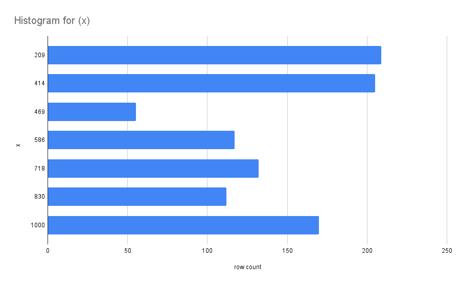
The ideal histogram uses a small amount of space to accurately estimate a wide variety of range scans.
For example, lets say we have a range query:
select count(*) from xy
where
  x < 100 OR
  x between 200 and 300 OR
  x > 800;
x values are unique and range from [0,1000] So we can do a little
math to estimate that the result of the query will be 100 + (300-200) +
(1000-800) = 100 + 100 + 200 = 400.
We would use a histogram to estimate this value by truncating buckets that fall outside of the filter ranges. The output of that process looks something like the chart below:
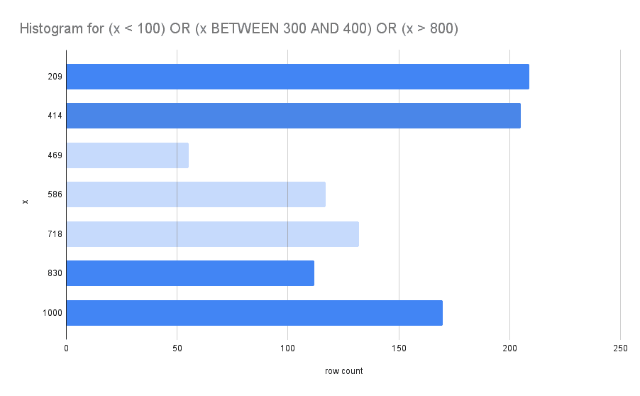
The sum of the remaining buckets is 696. This is not a perfect estimate of the query result, and histograms are not foolproof. But this is a lot better than zero information, and we at least have a trade-off where now we can add more buckets to get better estimates at the expense of maintaining a more expensive set of statistics.
More Complicated Example
Now we will do a more complicated example whose ideal index scan is less obvious.
This warehouse table has a unique identifier, geographical properties,
the date it started operating, and a maximum capacity. The table has a
few indexes that might reflect common access patterns.
CREATE warehouse (
  Id int primary key,
  City varchar(60),
  State varchar(60),
  Zip smallint,
  Region int,
  Capacity int,
  operatingStart datetime,
  Key (region, state, city, zip),
  Key (region, city, capacity),
  Key (operatingStart, capacity)
)
We consider a query that touches all three secondary indexes:
select * from warehouse
where
  region = 'North America' AND
  city = 'Lost Angeles' AND
  state = 'California' AND
  operatingStart >= '2022-01-01' AND
  capacity > 10;
In other words, a subset of filters are a partial match for each set of index column expression keys:
- ('North America', 'CA', 'Los Angeles', ?) => (region, state, city, zip)
- ('North America', 'CA', 10-∞) => (region, state, capacity)
- ('2022-01-01'-∞, ?) => (operatingStart, capacity)
(We number the options as a reference aid in the comparisons below)
-- option 1
(Project
  (*)
  (Filter
    (List
      (OperatingStart >= '2022-01-01')
      (Capacity > 10))
    (IndexScan
      (Index warehouse.regionStateCityZip)
      (Range ('North America') ('CA') ('Los Angeles') (-∞, ∞)))))

-- option 2
(Project
  (*)
  (Filter
    (List
      (City = 'Los Angeles')
      (OperatingStart >= '2022-01-01')
      (Capacity > 10))
    (IndexScan
      (Index warehouse.regionStateCapacity)
      (Range ('North America') ('CA') (10, ∞)))))

-- option 3
(Project
  (*)
  (Filter
    (List
      (Region = 'North America')
      (City = 'Los Angeles')
      (State = 'California')
      (Capacity > 10))
    (IndexScan
      (Index warehouse.operatingStartCapacity)
      (Range ('2022-01-01', ∞) (-∞, ∞)))))
Each index scan option has 1) a set of filters absorbed into the table scan, and 2) a remaining set of filters executed in memory. Depending on the contents of the database, all or none of these options might be fast.
If we skip a few steps, we can find the results of truncating the histograms for each index like we did above: (1) 1574, (2) 10002, (3) 345.
The range filter on operatingStart (option 3) is the most selective,
returns the fewest rows, and will be the most performant:
(Project
  (*)
  (Filter
    (List
      (Region = 'North America')
      (City = 'Los Angeles')
      (State = 'California')
      (Capacity > 10))
    (IndexScan
      (Index warehouse.operatingStartCapacity)
      (Range (-∞, '2020-01-01') (-∞, ∞)))))
It is important to keep in mind that changes to the database might
change the optimal index scan. For example, if several thousand new
warehouses became operational next year, suddenly operatingStart <
2022 will not be as competitive.
Future
We look forward to expanding costing to improve other optimizer decisions like join planning, sorting externally vs with an index, and choosing whether to aggregate before or after joins. We will also soon publish blogs talking more about the storage-layer lifecycle of Dolt statistics.
Until then, if you have any questions about Dolt, databases, or Golang performance reach out to us on Twitter, Discord, and GitHub!